如何绘制Python 3维水平集? [英] How to plot a Python 3-dimensional level set?
问题描述
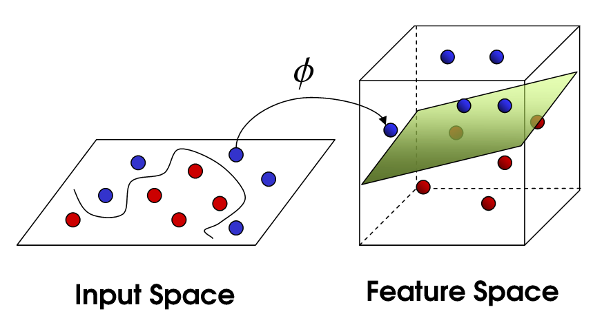
我在绘制脑海中的图像时遇到了一些麻烦.我想用支持向量机可视化内核技巧.所以我做了一些由两个圆(一个内圆和一个外圆)组成的二维数据,这两个圆应该被一个超平面分开.显然,这在二维上是不可能的-因此我将它们转换为3D.令n为样本数.现在我有一个 (n,3) 数组(3 列,n 行)X 的数据点和一个带标签的 (n,1) 数组 y.使用sklearn,我可以通过
获得线性分类器 clf = svm.SVC(内核='线性',C = 1000)clf.fit(X,y)我已经通过
将数据点绘制为散点图plt.scatter(X[:, 0], X[:, 1], c=y, s=30, cmap=plt.cm.Paired)现在我想将分离超平面绘制为曲面图.我的问题是缺少超平面的显式表示,因为决策函数仅通过 decision_function = 0 生成隐式超平面.因此我需要绘制一个 4 维对象的水平集(0 级).
由于我不是 Python 专家,如果有人能帮助我,我将不胜感激!而且我知道这并不是真正的样式".使用 SVM,但我需要这张图片作为我论文的插图.
我当前的代码"
将numpy导入为np导入matplotlib.pyplot作为plt从 sklearn 导入 svm从 sklearn.datasets 导入 make_blobs, make_circles从 tikzplotlib 导入另存为 tikz_saveplt.close('all')#我们创建50个可分离的点#X,y = make_blobs(n_samples = 40,centers = 2,random_state = 6)X,y = make_circles(n_samples = 50,factor = 0.5,random_state = 4,noise = .05)X2, y2 = make_circles(n_samples=50, factor=0.2, random_state=5, noise=.08)X = np.append(X,X2,轴= 0)y = np.append(y,y2,axis = 0)# 将 X 移到 [0,2]x[0,2]X = np.array([[item [0] + 1,item [1] + 1] for X in item]X [X <0] = 0.01clf = svm.SVC(kernel='rbf', C=1000)clf.fit(X,y)plt.scatter(X[:, 0], X[:, 1], c=y, s=30, cmap=plt.cm.Paired)#绘制决策函数ax = plt.gca()xlim = ax.get_xlim()ylim = ax.get_ylim()# 创建网格来评估模型xx = np.linspace(xlim[0], xlim[1], 30)yy = np.linspace(ylim [0],ylim [1],30)YY, XX = np.meshgrid(yy, xx)xy = np.vstack([XX.ravel(),YY.ravel()]).TZ = clf.decision_function(xy).reshape(XX.shape)# 绘制决策边界和边距ax.contour(XX, YY, Z, colors='k', levels=[-1, 0, 1], alpha=0.5, linestyles=['--','-','--'])# 绘制支持向量ax.scatter(clf.support_vectors_ [:, 0],clf.support_vectors_ [:, 1],s = 100,linewidth = 1,facecolors ="none",edgecolors ="k")################## 内核技巧 - 3D ##################trans_X = np.array([[[item [0] ** 2,item [1] ** 2,np.sqrt(2 * item [0] * item [1])]]无花果= plt.figure()ax = plt.axes(投影="3d")# 创建散点图ax.scatter3D(trans_X [:,0],trans_X [:,1],trans_X [:,2],c = y,cmap = plt.cm.Paired)clf2 = svm.SVC(内核='线性',C = 1000)clf2.fit(trans_X, y)ax = plt.gca(projection='3d')xlim = ax.get_xlim()ylim = ax.get_ylim()zlim = ax.get_zlim()###从这里我不知道该怎么做###xx = np.linspace(xlim [0],xlim [1],3)yy = np.linspace(ylim[0], ylim[1], 3)zz = np.linspace(zlim [0],zlim [1],3)ZZ,YY,XX = np.meshgrid(zz,yy,xx)xyz = np.vstack([XX.ravel(),YY.ravel(),ZZ.ravel()]).TZ = clf2.decision_function(xyz).reshape(XX.shape)#ax.contour(XX,YY,ZZ,Z,colors ='k',level = [-1,0,1],alpha = 0.5,linestyles = ['-','-','-'])所需的输出
我想要
脚注:使用 matplotlib 进行 3D 绘图
请注意,Matplotlib 3D无法管理深度"信息.在某些情况下对象的数量,因为它可能与此对象的 zorder 冲突.这就是为什么有时超平面看起来被绘制在之上"的原因.点,即使它应该落后".此问题是 matplotlib 3d文档和此答案.
如果您想获得更好的渲染结果,您可能需要使用 Mayavi,根据 Matplotlib 开发人员或任何其他 3D Python 绘图库的推荐.
I have some trouble plotting the image which is in my head. I want to visualize the Kernel-trick with Support Vector Machines. So I made some two-dimensional data consisting of two circles (an inner and an outer circle) which should be separated by a hyperplane. Obviously this isn't possible in two dimensions - so I transformed them into 3D. Let n be the number of samples. Now I have an (n,3)-array (3 columns, n rows) X of data points and an (n,1)-array y with labels. Using sklearn I get the linear classifier via
clf = svm.SVC(kernel='linear', C=1000)
clf.fit(X, y)
I already plot the data points as scatter plot via
plt.scatter(X[:, 0], X[:, 1], c=y, s=30, cmap=plt.cm.Paired)
Now I want to plot the separating hyperplane as surface plot. My problem here is the missing explicit representation of the hyperplane because the decision function only yields an implicit hyperplane via decision_function = 0. Therefore I need to plot the level set (of level 0) of an 4-dimensional object.
Since I'm not a python expert I would appreciate if somebody could help me out! And I know that this isn't really the "style" of using a SVM but I need this image as an illustration for my thesis.
Edit: my current "code"
import numpy as np
import matplotlib.pyplot as plt
from sklearn import svm
from sklearn.datasets import make_blobs, make_circles

from tikzplotlib import save as tikz_save

plt.close('all')

# we create 50 separable points
#X, y = make_blobs(n_samples=40, centers=2, random_state=6)
X,  y  = make_circles(n_samples=50, factor=0.5, random_state=4, noise=.05)
X2, y2 = make_circles(n_samples=50, factor=0.2, random_state=5, noise=.08)

X = np.append(X,X2, axis=0)
y = np.append(y,y2, axis=0)

# shifte X to [0,2]x[0,2]
X = np.array([[item[0] + 1, item[1] + 1] for item in X])
X[X<0] = 0.01

clf = svm.SVC(kernel='rbf', C=1000)
clf.fit(X, y)

plt.scatter(X[:, 0], X[:, 1], c=y, s=30, cmap=plt.cm.Paired)


# plot the decision function
ax = plt.gca()
xlim = ax.get_xlim()
ylim = ax.get_ylim()

# create grid to evaluate model
xx = np.linspace(xlim[0], xlim[1], 30)
yy = np.linspace(ylim[0], ylim[1], 30)
YY, XX = np.meshgrid(yy, xx)
xy = np.vstack([XX.ravel(), YY.ravel()]).T
Z = clf.decision_function(xy).reshape(XX.shape)

# plot decision boundary and margins
ax.contour(XX, YY, Z, colors='k', levels=[-1, 0, 1], alpha=0.5, linestyles=['--','-','--'])
# plot support vectors
ax.scatter(clf.support_vectors_[:, 0], clf.support_vectors_[:, 1], s=100,
           linewidth=1, facecolors='none', edgecolors='k')


################## KERNEL TRICK - 3D ##################

trans_X = np.array([[item[0]**2, item[1]**2, np.sqrt(2*item[0]*item[1])] for item in X])

fig = plt.figure()
ax = plt.axes(projection ="3d")

# creating scatter plot
ax.scatter3D(trans_X[:,0],trans_X[:,1],trans_X[:,2], c = y, cmap=plt.cm.Paired)

clf2 = svm.SVC(kernel='linear', C=1000)
clf2.fit(trans_X, y)


ax = plt.gca(projection='3d')
xlim = ax.get_xlim()
ylim = ax.get_ylim()
zlim = ax.get_zlim()

### from here i don't know what to do ###
xx = np.linspace(xlim[0], xlim[1], 3)
yy = np.linspace(ylim[0], ylim[1], 3)
zz = np.linspace(zlim[0], zlim[1], 3)
ZZ, YY, XX = np.meshgrid(zz, yy, xx)
xyz = np.vstack([XX.ravel(), YY.ravel(), ZZ.ravel()]).T
Z = clf2.decision_function(xyz).reshape(XX.shape)
#ax.contour(XX, YY, ZZ, Z, colors='k', levels=[-1, 0, 1], alpha=0.5, linestyles=['--','-','--'])
Desired Output
I want to get something like that. In general I want to reconstruct what they do in this article, especially "Non-linear transformations".
Part of your question is addressed in this question on linear-kernel SVM. It's a partial answer, because only linear kernels can be represented this way, i.e. thanks to hyperplane coordinates accessible via the estimator when using linear kernel.
Another solution is to find the isosurface with marching_cubes
This solution involves installing the scikit-image toolkit (https://scikit-image.org) which allows to find an isosurface of a given value (here, I considered 0 since it represents the distance to the hyperplane) from the mesh grid of the 3D coordinates.
In the code below (copied from yours), I implement the idea for any kernel (in the example, I used the RBF kernel), and the output is shown beneath the code. Please consider my footnote about 3D plotting with matplotlib, which may be another issue in your case.
import numpy as np
import matplotlib.pyplot as plt
from sklearn import svm
from skimage import measure
from sklearn.datasets import make_blobs, make_circles

from tikzplotlib import save as tikz_save
from mpl_toolkits.mplot3d.art3d import Poly3DCollection

plt.close('all')

# we create 50 separable points
#X, y = make_blobs(n_samples=40, centers=2, random_state=6)
X,  y  = make_circles(n_samples=50, factor=0.5, random_state=4, noise=.05)
X2, y2 = make_circles(n_samples=50, factor=0.2, random_state=5, noise=.08)

X = np.append(X,X2, axis=0)
y = np.append(y,y2, axis=0)

# shifte X to [0,2]x[0,2]
X = np.array([[item[0] + 1, item[1] + 1] for item in X])
X[X<0] = 0.01

clf = svm.SVC(kernel='rbf', C=1000)
clf.fit(X, y)

plt.scatter(X[:, 0], X[:, 1], c=y, s=30, cmap=plt.cm.Paired)


# plot the decision function
ax = plt.gca()
xlim = ax.get_xlim()
ylim = ax.get_ylim()

# create grid to evaluate model
xx = np.linspace(xlim[0], xlim[1], 30)
yy = np.linspace(ylim[0], ylim[1], 30)
YY, XX = np.meshgrid(yy, xx)
xy = np.vstack([XX.ravel(), YY.ravel()]).T
Z = clf.decision_function(xy).reshape(XX.shape)

# plot decision boundary and margins
ax.contour(XX, YY, Z, colors='k', levels=[-1, 0, 1], alpha=0.5, linestyles=['--','-','--'])
# plot support vectors
ax.scatter(clf.support_vectors_[:, 0], clf.support_vectors_[:, 1], s=100,
           linewidth=1, facecolors='none', edgecolors='k')


################## KERNEL TRICK - 3D ##################

trans_X = np.array([[item[0]**2, item[1]**2, np.sqrt(2*item[0]*item[1])] for item in X])

fig = plt.figure()
ax = plt.axes(projection ="3d")

# creating scatter plot
ax.scatter3D(trans_X[:,0],trans_X[:,1],trans_X[:,2], c = y, cmap=plt.cm.Paired)

clf2 = svm.SVC(kernel='rbf', C=1000)
clf2.fit(trans_X, y)


z = lambda x,y: (-clf2.intercept_[0]-clf2.coef_[0][0]*x-clf2.coef_[0][1]*y) / clf2.coef_[0][2]

ax = plt.gca(projection='3d')
xlim = ax.get_xlim()
ylim = ax.get_ylim()
zlim = ax.get_zlim()

### from here i don't know what to do ###
xx = np.linspace(xlim[0], xlim[1], 50)
yy = np.linspace(ylim[0], ylim[1], 50)
zz = np.linspace(zlim[0], zlim[1], 50)
XX ,YY, ZZ = np.meshgrid(xx, yy, zz)
xyz = np.vstack([XX.ravel(), YY.ravel(), ZZ.ravel()]).T
Z = clf2.decision_function(xyz).reshape(XX.shape)

# find isosurface with marching cubes
dx = xx[1] - xx[0]
dy = yy[1] - yy[0]
dz = zz[1] - zz[0]
verts, faces, _, _ = measure.marching_cubes_lewiner(Z, 0, spacing=(1, 1, 1), step_size=2)
verts *= np.array([dx, dy, dz])
verts -= np.array([xlim[0], ylim[0], zlim[0]])

# add as Poly3DCollection
mesh = Poly3DCollection(verts[faces])
mesh.set_facecolor('g')
mesh.set_edgecolor('none')
mesh.set_alpha(0.3)
ax.add_collection3d(mesh)
ax.view_init(20, -45)
plt.savefig('kerneltrick')
Running the code produces the following image with Matplotlib, where the green semi-transparent surface represents the non-linear decision boundary.
Footnote: 3D plotting with matplotlib
Note that Matplotlib 3D is not able to manage the "depth" of objects in some cases, because it can be in conflict with the zorder of this object. This is the reason why sometimes the hyperplane look to be plotted "on top of" the points, even it should be "behind". This issue is a known bug discussed in the matplotlib 3d documentation and in this answer.
If you want to have better rendering results, you may want to use Mayavi, as recommended by the Matplotlib developers, or any other 3D Python plotting library.
这篇关于如何绘制Python 3维水平集?的文章就介绍到这了,希望我们推荐的答案对大家有所帮助,也希望大家多多支持IT屋!
