边界椭圆 [英] Bounding ellipse
问题描述
这是使用AWT形状在java(euch)中工作的,所以我可以使用所有形状提供的工具来检查包含/交叉对象。
您正在寻找并不保证从分解中得到的椭圆( eigen /奇异值)将是椭圆的最小边界,因为椭圆外的点表示变化。
<编辑:
因此,如果有人阅读文档,有两种方法可以在2D中进行:这是最佳的伪代码算法 - 次优算法在文档中有明确的解释:
$ b 最佳算法:
 输入:存储10个二维点
且容差为误差的2x10矩阵P.
输出:矩阵形式的椭圆公式,即
,即一个2×2矩阵A和一个2×1矢量C,表示
是椭圆的中心。

 //点的维数
 d = 2;
 //点数
 N = 10;

 //向2xN矩阵P添加一行1,所以Q现在是3xN。
 Q = [P; ones(1,N)]

 //初始化
 count = 1;
 err = 1;
 // u是一个Nx1向量,其中每个元素为1 / N
u =(1 / N)* ones(N,1)

 // Khachiyan算法
而错误>容差
 {
 //矩阵乘法:
 // diag(u):如果u是一个向量,则将u
 //的元素放在NxN矩阵的对角线上零
 X = Q * diag(u)* Q'; // Q' - 转置的Q

 // inv(X)返回矩阵的逆矩阵X
 // diag(M)当M是矩阵时,返回对角线向量M
 M = diag(Q'* inv(X)* Q); // Q' - 转置Q

 //找到向量中最大元素的值和位置M
 maximum = max(M);
 j = find_maximum_value_location(M);

 //计算上升的步长
 step_size =(maximum -d -1)/((d + 1)*(maximum-1));

 //计算new_u:
 //取出向量u,并将其中的所有元素乘以(1-step_size)
 new_u =(1  -  step_size)*你

 //通过step_size增加new_u的第j个元素
 new_u(j)= new_u(j)+ step_size;

 //通过查找SSD的平方根存储错误
 // new_u和u
之间// SSD或平方和差值两个相同大小的向量
 //创建一个新向量,方法是找到相应元素之间的
 //差值,并将
 //每个差值平方并将它们相加。

 //所以如果向量是:a = [1 2 3]和b = [5 4 6],那么:
 // SSD =(1-5)^ 2 + (2-4)^ 2 +(3-6)^ 2;
 //规范(a-b)= sqrt(SSD);
 err = norm(new_u  -  u);

 //递增计数并替换u
 count = count + 1;
 u = new_u;
}

 //将矢量u的元素放入矩阵
 // U的对角线中,其余元素为0
 U = diag (U);

 //计算A矩阵
 A =(1 / d)* inv(P * U * P' - (P * u)*(P * u)');

 //中心,
 c = P * u;
I have been given an assignement for a graphics module, one part of which is to calculate the minimum bounding ellipse of a set of arbitrary shapes. The ellipse doesn't have to be axis aligned.
This is working in java (euch) using the AWT shapes, so I can use all the tools shape provides for checking containment/intersection of objects.
You're looking for the Minimum Volume Enclosing Ellipsoid, or in your 2D case, the minimum area. This optimization problem is convex and can be solved efficiently. Check out the MATLAB code in the link I've included - the implementation is trivial and doesn't require anything more complex than a matrix inversion.
Anyone interested in the math should read this document.
Also, plotting the ellipse is also simple - this can be found here, but you'll need a MATLAB-specific function to generate points on the ellipse.
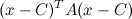
But since the algorithm returns the equation of the ellipse in the matrix form,
matrix form http://mathurl.com/yz7flxe.png
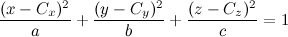
you can use this code to see how you can convert the equation to the canonical form,
canonical http://mathurl.com/y86tlbw.png
using Singular Value Decomposition (SVD). And then it's quite easy to plot the ellipse using the canonical form.
Here's the result of the MATLAB code on a set of 10 random 2D points (blue).
Other methods like PCA does not guarantee that the ellipse obtained from the decomposition (eigen/singular value) will be minimum bounding ellipse since points outside the ellipse is an indication of the variance.
EDIT:
So if anyone read the document, there are two ways to go about this in 2D: here's the pseudocode of the optimal algorithm - the suboptimal algorithm is clearly explained in the document:
Optimal algorithm:
Input: A 2x10 matrix P storing 10 2D points
       and tolerance = tolerance for error.
Output: The equation of the ellipse in the matrix form,
        i.e. a 2x2 matrix A and a 2x1 vector C representing
        the center of the ellipse.

// Dimension of the points
d = 2;
// Number of points
N = 10;

// Add a row of 1s to the 2xN matrix P - so Q is 3xN now.
Q = [P;ones(1,N)]

// Initialize
count = 1;
err = 1;
//u is an Nx1 vector where each element is 1/N
u = (1/N) * ones(N,1)

// Khachiyan Algorithm
while err > tolerance
{
    // Matrix multiplication:
    // diag(u) : if u is a vector, places the elements of u
    // in the diagonal of an NxN matrix of zeros
    X = Q*diag(u)*Q'; // Q' - transpose of Q

    // inv(X) returns the matrix inverse of X
    // diag(M) when M is a matrix returns the diagonal vector of M
    M = diag(Q' * inv(X) * Q); // Q' - transpose of Q

    // Find the value and location of the maximum element in the vector M
    maximum = max(M);
    j = find_maximum_value_location(M);

    // Calculate the step size for the ascent
    step_size = (maximum - d -1)/((d+1)*(maximum-1));

    // Calculate the new_u:
    // Take the vector u, and multiply all the elements in it by (1-step_size)
    new_u = (1 - step_size)*u ;

    // Increment the jth element of new_u by step_size
    new_u(j) = new_u(j) + step_size;

    // Store the error by taking finding the square root of the SSD
    // between new_u and u
    // The SSD or sum-of-square-differences, takes two vectors
    // of the same size, creates a new vector by finding the
    // difference between corresponding elements, squaring
    // each difference and adding them all together.

    // So if the vectors were: a = [1 2 3] and b = [5 4 6], then:
    // SSD = (1-5)^2 + (2-4)^2 + (3-6)^2;
    // And the norm(a-b) = sqrt(SSD);
    err = norm(new_u - u);

    // Increment count and replace u
    count = count + 1;
    u = new_u;
}

// Put the elements of the vector u into the diagonal of a matrix
// U with the rest of the elements as 0
U = diag(u);

// Compute the A-matrix
A = (1/d) * inv(P * U * P' - (P * u)*(P*u)' );

// And the center,
c = P * u;
这篇关于边界椭圆的文章就介绍到这了,希望我们推荐的答案对大家有所帮助,也希望大家多多支持IT屋!
