Google工作表：将工作表1中的单元格值与工作表2列中的单元格值进行比较 [英] Google sheets: Compare cell value in sheet 1 to cell values in a column of sheet 2

问题描述

我在一个文件中有2个工作表。每张表中的栏目A都有一个网站列表。当我在表格1的栏目A中输入一个新网站时，我需要它将表格与表格2中的表格进行比较。

I have a 2 worksheets within a single file. Col A in each sheet has a list of websites. When I enter a new website to col A of sheet 1, I need it to compare the entry to the list on sheet 2.

如果同一个网站在表格中列出2，我需要以某种方式标记新条目 - 红色背景，粗体，任何。

If the same website is listed on sheet 2, I need the new entry to be marked in some way - red background, bolded, whatever.

它应该是什么样子：

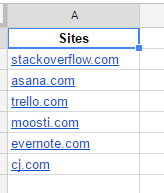
工作表1：
https://i.gyazo.com/ 07667520bc0f58a1dd2547405545eb5e.png

表2：
https://i.gyazo.com/a524832a9cb96e35bd2981e95e5c1edf.png

Stackoverflow在表2中列出，所以当它被添加到工作表1它被标记为红色。

Stackoverflow is listed on sheet 2, so when it's added to sheet 1 it's marked with red.

我一直在谷歌搜索和检查SO线程大约一个小时，但我甚至无法开始解决这个问题。我对这种东西的经验很少。

I've been Googling and checking SO threads for about an hour, but I can't even begin to figure this out. I have very little experience with this stuff.

任何帮助表示赞赏。感谢！

Any help appreciated. Thanks!

推荐答案

格式>有条件格式
然后设置格式化规则，包括单元格值在内的选项'等于'
它应该有效。

It may be possible with Format>Conditional Formatting then set a Rule for formatting, there are many options including cell value 'equal to' It should work.

这篇关于Google工作表：将工作表1中的单元格值与工作表2列中的单元格值进行比较的文章就介绍到这了，希望我们推荐的答案对大家有所帮助，也希望大家多多支持IT屋！