R - 时间序列分析

时间序列是一系列数据点，其中每个数据点与时间戳相关联.一个简单的例子是股票市场中某一天的不同时间点的股票价格.另一个例子是一年中不同月份的一个地区的降雨量. R语言使用许多函数来创建，操作和绘制时间序列数据.时间序列的数据存储在名为时间序列对象的R对象中.它也是一个R数据对象，如矢量或数据框.

时间序列对象是使用 ts()函数创建的.

语法

时间序列分析中 ts()函数的基本语法是 :

timeseries.object.name <-  ts(data, start, end, frequency)

以下是使用参数的描述;

• 数据是包含值的向量或矩阵在时间序列中使用.

• start 指定第一次观察的时间序列的开始时间.

• 结束指定上次观察时间序列的结束时间.

• 频率指定每单位时间的观察次数.

除参数"data"外，所有其他参数均为可选.

示例

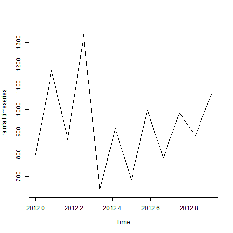
考虑年降雨量de从2012年1月开始的一个地方的尾巴.我们创建一个R时间序列对象为期12个月并绘制它.

# Get the data points in form of a R vector.
rainfall <- c(799,1174.8,865.1,1334.6,635.4,918.5,685.5,998.6,784.2,985,882.8,1071)

# Convert it to a time series object.
rainfall.timeseries <- ts(rainfall,start = c(2012,1),frequency = 12)

# Print the timeseries data.
print(rainfall.timeseries)

# Give the chart file a name.
png(file = "rainfall.png")

# Plot a graph of the time series.
plot(rainfall.timeseries)

# Save the file.
dev.off()

当我们执行上面的代码时，它会产生以下结果和图表 :

Jan    Feb    Mar    Apr    May     Jun    Jul    Aug    Sep
2012  799.0  1174.8  865.1  1334.6  635.4  918.5  685.5  998.6  784.2
        Oct    Nov    Dec
2012  985.0  882.8 1071.0

时间序列图表 : 去;

不同时间间隔

ts()中频率参数的值函数决定测量数据点的时间间隔.值12表示时间序列为12个月.其他值及其含义如下:<

• frequency = 12 查看数据点一年中的每个月.

• 频率= 4 固定一年中每个季度的数据点.

• 频率= 6 每10分钟固定一次数据点.

• 频率= 24 * 6 每天每10分钟固定数据点.

多个时间序列

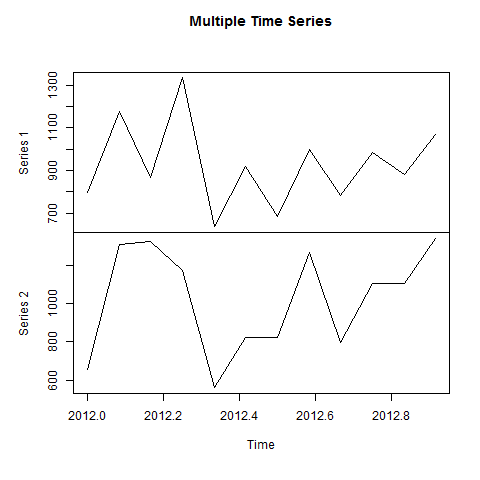
我们可以通过将两个系列组合成一个矩阵，在一个图表中绘制多个时间序列.

# Get the data points in form of a R vector.
rainfall1 <- c(799,1174.8,865.1,1334.6,635.4,918.5,685.5,998.6,784.2,985,882.8,1071)
rainfall2 <- 
           c(655,1306.9,1323.4,1172.2,562.2,824,822.4,1265.5,799.6,1105.6,1106.7,1337.8)

# Convert them to a matrix.
combined.rainfall <-  matrix(c(rainfall1,rainfall2),nrow = 12)

# Convert it to a time series object.
rainfall.timeseries <- ts(combined.rainfall,start = c(2012,1),frequency = 12)

# Print the timeseries data.
print(rainfall.timeseries)

# Give the chart file a name.
png(file = "rainfall_combined.png")

# Plot a graph of the time series.
plot(rainfall.timeseries, main = "Multiple Time Series")

# Save the file.
dev.off()

当我们执行上面的代码时，它会产生以下结果和图表 :

           Series 1  Series 2
Jan 2012    799.0    655.0
Feb 2012   1174.8   1306.9
Mar 2012    865.1   1323.4
Apr 2012   1334.6   1172.2
May 2012    635.4    562.2
Jun 2012    918.5    824.0
Jul 2012    685.5    822.4
Aug 2012    998.6   1265.5
Sep 2012    784.2    799.6
Oct 2012    985.0   1105.6
Nov 2012    882.8   1106.7
Dec 2012   1071.0   1337.8

多次时间序列图表 : 去;