GraphPlots 的大小一致 [英] Consistent size for GraphPlots
问题描述
10/27 更新:我已经在答案中提供了实现一致规模的详细步骤.基本上对于每个 Graphics 对象,您需要将所有填充/边距固定为 0 并手动指定 plotRange 和 imageSize,以便 1) plotRange 包括所有图形 2) imageSize=scale*plotRange
现在仍然确定如何做 1) 完全通用,给出了适用于由点和粗线组成的图形 (AbsoluteThickness) 的解决方案
<小时>我在 VertexRenderingFunction 和VertexCoordinates"中使用Inset"来保证图的子图之间的外观一致.使用Inset"将这些子图绘制为另一个图的顶点.有两个问题,一个是生成的框没有围绕图裁剪(即一个顶点的图仍然放在一个大框中),另一个是大小之间存在奇怪的变化(你可以看到一个框是垂直的).有人能找到解决这些问题的方法吗?
这与之前的
(来源:
(来源:
(来源:yaroslavvb.com)
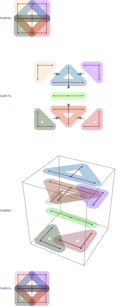
(**** 注意,这里使用了 Mathematica 8 基元 JoinedCurve 和 Texture.在 Mathematica 7 中,JoinedCurve 不需要,可以删除 *)(** 全局变量 **)规模 = 50;线厚 = 1/2;(* 常规坐标中的线条粗细 *)(** 全局实用程序 **)(* 测试 3 个点是否共线,需要解决差异 \在如何呈现共线线端点 *)共线[点数_] :=长度[点数] == 3 &&(Det[Transpose[points]~Append~{1, 1, 1}] == 0)(* 故事点坐标列表,返回 plotRange 边界框,\使用全局scale"和lineThickness"来获取边界框 *)getPlotRange[lst_] := ({xs, ys} = 转置 [lst];(* 两个额外的 1/精确匹配所需的比例偏移 *){{Min[xs] -线厚/2,Max[xs] + lineThickness/2 + 1/scale}, {Min[ys] -lineThickness/2 - 1/scale, Max[ys] + lineThickness/2}});(* 获取给定绘图范围的图像大小 *)getImageSize[{{xmin_, xmax_}, {ymin_, ymax_}}] := (imsize = scale*{xmax - xmin, ymax - ymin} + {1, 1});(* 将绘图范围转换为矩形的顶点 *)pr2verts[{{xmin_, xmax_}, {ymin_, ymax_}}] := {{xmin, ymin}, {xmax,ymin}, {xmax, ymax}, {xmin, ymax}};(* 将二维坐标提升为 3d *)Lift[h_, coords_] := Append[#, h] &/@ 坐标(* 将 Raster 对象转换为纹理的数组规范 *)raster2texture[raster_] := 反向[raster[[1, 1]]/255]子集[a_, b_] := (a \[Intersection] b == a);诱导图[set_] := Select[edges, # \[Subset] set &];values[dict_] := Map[#[[-1]] &, DownValues[dict]];(** 图形特定的东西 *)graphName = {"网格", {3, 3}};verts = Range[GraphData[graphName, "VertexCount"]];边 = GraphData[graphName, "EdgeIndices"];vcoords = Thread[verts ->GraphData[graphName, "顶点坐标"]];jedges = {{{1, 2, 4}, {2, 4, 5, 6}}, {{2, 3, 6}, {2, 4, 5, 6}}, {{4,5, 6}, {2, 4, 5, 6}}, {{4, 5, 6}, {4, 5, 6, 8}}, {{4, 7, 8}, {4,5, 6, 8}}, {{6, 8, 9}, {4, 5, 6, 8}}};jnodes = Union[Flatten[jedges, 1]];(* 使用显式 PlotRange、ImageSize 和 \ 生成图表绝对厚度 *)plotHL[verts_, color_] := (坐标 = verts/.坐标;obj = JoinedCurve[线[坐标],CurveClosed ->不[共线[坐标]]];(* 计算出遵守比例所需的 PlotRange 和 ImageSize *)pr = getPlotRange[verts/.坐标];{{xmin, xmax}, {ymin, ymax}} = pr;imsize = scale*{xmax - xmin, ymax - ymin};lineForm = {Opacity[.3], color, JoinForm["Round"],CapForm["Round"], AbsoluteThickness[scale*lineThickness]};g = 图形[{Directive[lineForm], obj}];gg = GraphPlot[规则@@@inducedGraph[verts],顶点坐标规则 ->坐标];显示[g, gg, PlotRange ->pr,图像大小 ->大小]);(* 初始化所有图形绘图图像 *)种子随机[1];颜色 =RandomChoice[ColorData["WebSafe", "ColorList"], Length[jnodes]];清除[袋];MapThread[(bags[#1] = plotHL[#1, #2]) &, {jnodes, colors}];(** 绘制子图的父图 **)(* 找出靠近边界边缘的子图的坐标 \框,使用它们来锚定父 GraphPlot *)bagCentroid[bag_] := 平均值[bag/.坐标];findExtremeBag[vec_] := (vertList = First/@ vcoords;coordList = Last/@ vcoords;极端位置 =首先[排序[jnodes, 1,bagCentroid[#1].vec >bagCentroid[#2].vec &]];jnodes[[extremePos]]);ExtremeDirs = {{1, 1}, {1, -1}, {-1, 1}, {-1, -1}};ExtremeBags = findExtremeBag//@extremeDirs;ExtremePoses = bagCentroid//@extremeBags;(* 找出包含所有对象所需的新绘图范围 *)fullPR = getPlotRange[verts/.坐标];fullIS = getImageSize[fullPR];(*** 显示包合并在一起 ***)图像 1 =Show[values[bags], PlotRange ->fullPR, ImageSize ->完整的](*** 将包显示为另一个 GraphPlot 的顶点 ***)GraphPlot[规则@@@ jedges,EdgeRenderingFunction ->({灰色,粗,箭头[.05],箭头 [#1, 0.22]} &),顶点坐标规则 ->线程[线程[extremeBags ->极端姿势]],VertexRenderingFunction ->(插入[袋子[#2], #] &),绘图范围 ->全公关,图像大小 ->3*全IS](*** 以 3d 幻灯片形式显示包 ***)makeSlide[graphics_, pr_, h_] := (Graphics3D[{纹理[raster2texture[光栅化[图形,背景 ->没有任何]]],EdgeForm[无],多边形[lift[h, pr2verts[pr]],顶点纹理坐标 ->pr2verts[{{0, 1}, {0, 1}}]]}])yoffset = 1/2;幻灯片 = MapIndexed[makeSlide[bags[#], getPlotRange[#/.坐标],yoffset*First[#2]] &, jnodes];显示[幻灯片,图像大小 ->3*fullIS](*** 在正交投影中显示 3d 幻灯片 ***)图像 2 =显示[幻灯片,视点 ->{0, 0, Infinity}, ImageSize ->完整的,盒装 ->错误的](*** 检查 3d 和 2d 图像是否光栅化为相同的分辨率 ***)尺寸[光栅化[图像1][[1, 1]]] ==尺寸[光栅化[图像2][[1, 1]]]Update 10/27: I've put detailed steps for achieving consistent scale in an answer. Basically for each Graphics object you need to fix all padding/margins to 0 and manually specify plotRange and imageSize that such that 1) plotRange includes all graphics 2) imageSize=scale*plotRange
Still now sure how to do 1) in full generality, a solution that works for Graphics consisting of points and thick lines (AbsoluteThickness) is given
I'm using "Inset" in VertexRenderingFunction and "VertexCoordinates" to guarantee consistent appearance among subgraphs of a graph. Those subgraphs are drawn as vertices of another graph, using "Inset". There are two problems, one is that resulting boxes are not cropped around the graph (ie, graph with one vertex still gets placed in a big box), and another is that there's strange variation among sizes (you can see one box is vertical). Can anyone see a way around these problems?
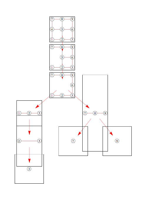
This is related to an earlier question of how to keep vertex sizes looking the same, and while Michael Pilat's suggestion of using Inset works to keep vertices rendering at the same scale, overall scale may be different. For instance on the left branch, the graph consisting of vertices 2,3 is stretched relative to the "2,3" subgraph in the top graph, even though I'm using absolute vertex positioning for both
(source: yaroslavvb.com)
(*utilities*)intersect[a_, b_] := Select[a, MemberQ[b, #] &];
induced[s_] := Select[edges, #~intersect~s == # &];
Needs["GraphUtilities`"];
subgraphs[
   verts_] := (gr =
    Rule @@@ Select[edges, (Intersection[#, verts] == #) &];
   Sort /@ WeakComponents[gr~Join~(# -> # & /@ verts)]);

(*graph*)
gname = {"Grid", {3, 3}};
edges = GraphData[gname, "EdgeIndices"];
nodes = Union[Flatten[edges]];
AppendTo[edges, #] & /@ ({#, #} & /@ nodes);
vcoords = Thread[nodes -> GraphData[gname, "VertexCoordinates"]];

(*decompose*)
edgesOuter = {};
pr[_, _, {}] := None;
pr[root_, elim_,
   remain_] := (If[root != {}, AppendTo[edgesOuter, root -> remain]];
   pr[remain, intersect[Rest[elim], #], #] & /@
    subgraphs[Complement[remain, {First[elim]}]];);
pr[{}, {4, 5, 6, 1, 8, 2, 3, 7, 9}, nodes];

(*visualize*)

vrfInner =
  Inset[Graphics[{White, EdgeForm[Black], Disk[{0, 0}, .05], Black,
      Text[#2, {0, 0}]}, ImageSize -> 15], #] &;
vrfOuter =
  Inset[GraphPlot[Rule @@@ induced[#2],
     VertexRenderingFunction -> vrfInner,
     VertexCoordinateRules -> vcoords, SelfLoopStyle -> None,
     Frame -> True, ImageSize -> 100], #] &;
TreePlot[edgesOuter, Automatic, nodes,
 EdgeRenderingFunction -> ({Red, Arrow[#1, 0.2]} &),
 VertexRenderingFunction -> vrfOuter, ImageSize -> 500]
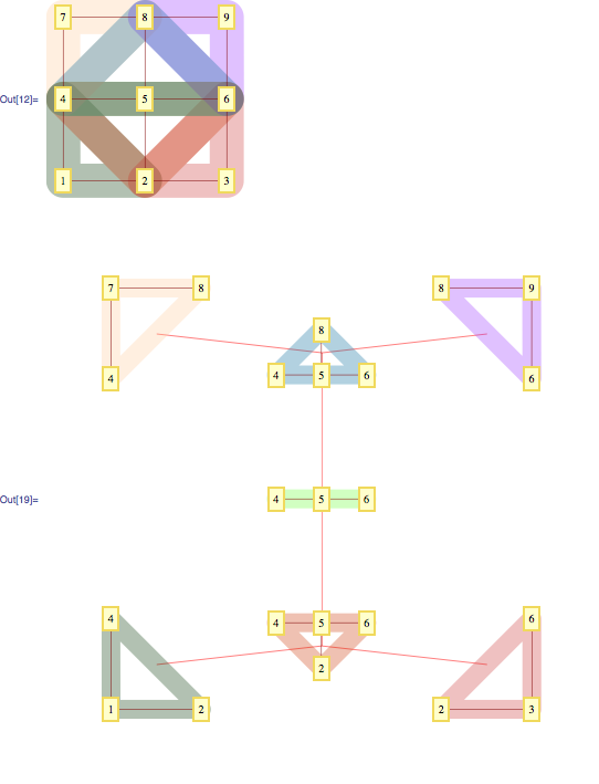
Here's another example, same problem as before, but the difference in relative scales is more visible. The goal is to have parts in the second picture match precisely the parts in the first picture.
(source: yaroslavvb.com)
(* Visualize tree decomposition of a 3x3 grid *)

inducedGraph[set_] := Select[edges, # \[Subset] set &];
Subset[a_, b_] := (a \[Intersection] b == a);
graphName = {"Grid", {3, 3}};
edges = GraphData[graphName, "EdgeIndices"];
vars = Range[GraphData[graphName, "VertexCount"]];
vcoords = Thread[vars -> GraphData[graphName, "VertexCoordinates"]];

plotHighlight[verts_, color_] := Module[{vpos, coords},
   vpos =
    Position[Range[GraphData[graphName, "VertexCount"]],
     Alternatives @@ verts];
   coords = Extract[GraphData[graphName, "VertexCoordinates"], vpos];
   If[coords != {}, AppendTo[coords, First[coords] + .002]];
   Graphics[{color, CapForm["Round"], JoinForm["Round"],
     Thickness[.2], Opacity[.3], Line[coords]}]];

jedges = {{{1, 2, 4}, {2, 4, 5, 6}}, {{2, 3, 6}, {2, 4, 5, 6}}, {{4,
     5, 6}, {2, 4, 5, 6}}, {{4, 5, 6}, {4, 5, 6, 8}}, {{4, 7, 8}, {4,
     5, 6, 8}}, {{6, 8, 9}, {4, 5, 6, 8}}};
jnodes = Union[Flatten[jedges, 1]];

SeedRandom[1]; colors =
 RandomChoice[ColorData["WebSafe", "ColorList"], Length[jnodes]];
bags = MapIndexed[plotHighlight[#, bc[#] = colors[[First[#2]]]] &,
   jnodes];
Show[bags~
  Join~{GraphPlot[Rule @@@ edges, VertexCoordinateRules -> vcoords,
    VertexLabeling -> True]}, ImageSize -> Small]

bagCentroid[bag_] := Mean[bag /. vcoords];
findExtremeBag[vec_] := (
   vertList = First /@ vcoords;
   coordList = Last /@ vcoords;
   extremePos =
    First[Ordering[jnodes, 1,
      bagCentroid[#1].vec > bagCentroid[#2].vec &]];
   jnodes[[extremePos]]
   );

extremeDirs = {{1, 1}, {1, -1}, {-1, 1}, {-1, -1}};
extremeBags = findExtremeBag /@ extremeDirs;
extremePoses = bagCentroid /@ extremeBags;
vrfOuter =
  Inset[Show[plotHighlight[#2, bc[#2]],
     GraphPlot[Rule @@@ inducedGraph[#2],
      VertexCoordinateRules -> vcoords, SelfLoopStyle -> None,
      VertexLabeling -> True], ImageSize -> 100], #] &;

GraphPlot[Rule @@@ jedges, VertexRenderingFunction -> vrfOuter,
 EdgeRenderingFunction -> ({Red, Arrowheads[0], Arrow[#1, 0]} &),
 ImageSize -> 500,
 VertexCoordinateRules -> Thread[Thread[extremeBags -> extremePoses]]]
Any other suggestions for aesthetically pleasing visualization of graph operations are welcome.
Here are the steps needed to achieve precise control over relative scales of graphics objects.
To achieve consistent scale one needs to explicitly specify input coordinate range (regular coordinates) and output coordinate range (absolute coordinates). Regular coordinate range depends on PlotRange, PlotRangePadding (and possibly others options?). Absolute coordinate range depends on ImageSize,ImagePadding (and possibly other options?). For GraphPlot, it is sufficient to specify PlotRange and ImageSize.
To create Graphics object that renders at a pre-determined scale, you need to figure out PlotRange needed to fully include the object, corresponding ImageSize and return Graphics object with these settings specified. To figure out the necessary PlotRange when thick lines are involved it is easier to deal with AbsoluteThickness, call it abs. To fully include those lines you could take the smallest PlotRange that includes endpoints, then offset minimum x and maximum y boundaries by abs/2, and offset maximum x and minimum y boundaries by (abs/2+1). Note that these are output coordinates.
When combining several scale-calibrated Graphics objects you need to recalculate PlotRange/ImageSize and set them explicitly for the combined Graphics object.
To Inset scale-calibrated objects into GraphPlot you need to make sure that coordinates used for automatic GraphPlot positioning are in the same range. For that, you could pick several corner nodes, fix their positions manually, and let automatic positioning do the rest.
Primitives Line/JoinedCurve/FilledCurve render joins/caps differently depending on whether the line is (almost) collinear, so one needs to manually detect collinearity.
Using this approach, rendered images should have width equal to
(inputPlotRange*scale + 1) + lineThickness*scale + 1
First extra 1 is to avoid the "fencepost error" and second extra 1 is the extra pixel needed to add on the right to make sure thick lines are not cut-off
I've verified this formula by doing Rasterize on combined Show and rasterizing a 3D plot with objects mapped using Texture and viewed with Orthographic projection and it matches the predicted result. Doing 'Copy/Paste' on objects Inset into GraphPlot, and then Rasterizing, I get an image that's one pixel thinner than predicted.
(source: yaroslavvb.com)
(**** Note, this uses JoinedCurve and Texture which are Mathematica 8 primitives.
      In Mathematica 7, JoinedCurve is not needed and can be removed *)

(** Global variables **)
scale = 50;
lineThickness = 1/2; (* line thickness in regular coordinates *)

(** Global utilities **)

(* test if 3 points are collinear, needed to work around difference \
in how colinear Line endpoints are rendered *)

collinear[points_] :=
 Length[points] == 3 && (Det[Transpose[points]~Append~{1, 1, 1}] == 0)

(* tales list of point coordinates, returns plotRange bounding box, \
uses global "scale" and "lineThickness" to get bounding box *)

getPlotRange[lst_] := (
   {xs, ys} = Transpose[lst];
   (* two extra 1/
   scale offsets needed for exact match *)
   {{Min[xs] -
      lineThickness/2,
     Max[xs] + lineThickness/2 + 1/scale}, {Min[ys] -
      lineThickness/2 - 1/scale, Max[ys] + lineThickness/2}}
   );

(* Gets image size for given plot range *)

getImageSize[{{xmin_, xmax_}, {ymin_, ymax_}}] := (
   imsize = scale*{xmax - xmin, ymax - ymin} + {1, 1}
   );

(* converts plot range to vertices of rectangle *)

pr2verts[{{xmin_, xmax_}, {ymin_, ymax_}}] := {{xmin, ymin}, {xmax,
    ymin}, {xmax, ymax}, {xmin, ymax}};

(* lifts two dimensional coordinates into 3d *)

lift[h_, coords_] := Append[#, h] & /@ coords
(* convert Raster object to array specification of texture *)

raster2texture[raster_] := Reverse[raster[[1, 1]]/255]

Subset[a_, b_] := (a \[Intersection] b == a);
inducedGraph[set_] := Select[edges, # \[Subset] set &];
values[dict_] := Map[#[[-1]] &, DownValues[dict]];


(** Graph Specific Stuff *)
graphName = {"Grid", {3, 3}};
verts = Range[GraphData[graphName, "VertexCount"]];
edges = GraphData[graphName, "EdgeIndices"];
vcoords = Thread[verts -> GraphData[graphName, "VertexCoordinates"]];
jedges = {{{1, 2, 4}, {2, 4, 5, 6}}, {{2, 3, 6}, {2, 4, 5, 6}}, {{4,
     5, 6}, {2, 4, 5, 6}}, {{4, 5, 6}, {4, 5, 6, 8}}, {{4, 7, 8}, {4,
     5, 6, 8}}, {{6, 8, 9}, {4, 5, 6, 8}}};
jnodes = Union[Flatten[jedges, 1]];


(* Generate diagram with explicit PlotRange,ImageSize and \
AbsoluteThickness *)
plotHL[verts_, color_] := (
   coords = verts /. vcoords;
   obj = JoinedCurve[Line[coords],
     CurveClosed -> Not[collinear[coords]]];

   (* Figure out PlotRange and ImageSize needed to respect scale *)

    pr = getPlotRange[verts /. vcoords];
   {{xmin, xmax}, {ymin, ymax}} = pr;
   imsize = scale*{xmax - xmin, ymax - ymin};
   lineForm = {Opacity[.3], color, JoinForm["Round"],
     CapForm["Round"], AbsoluteThickness[scale*lineThickness]};
   g = Graphics[{Directive[lineForm], obj}];
   gg = GraphPlot[Rule @@@ inducedGraph[verts],
     VertexCoordinateRules -> vcoords];
   Show[g, gg, PlotRange -> pr, ImageSize -> imsize]
   );

(* Initialize all graph plot images *)
SeedRandom[1]; colors =
 RandomChoice[ColorData["WebSafe", "ColorList"], Length[jnodes]];
Clear[bags];
MapThread[(bags[#1] = plotHL[#1, #2]) &, {jnodes, colors}];

(** Ploting parent graph of subgraphs **)

(* figure out coordinates of subgraphs close to edges of bounding \
box, use them to anchor parent GraphPlot *)

bagCentroid[bag_] := Mean[bag /. vcoords];
findExtremeBag[vec_] := (vertList = First /@ vcoords;
   coordList = Last /@ vcoords;
   extremePos =
    First[Ordering[jnodes, 1,
      bagCentroid[#1].vec > bagCentroid[#2].vec &]];
   jnodes[[extremePos]]);

extremeDirs = {{1, 1}, {1, -1}, {-1, 1}, {-1, -1}};
extremeBags = findExtremeBag /@ extremeDirs;
extremePoses = bagCentroid /@ extremeBags;

(* figure out new plot range needed to contain all objects *)

fullPR = getPlotRange[verts /. vcoords];
fullIS = getImageSize[fullPR];

(*** Show bags together merged ***)
image1 =
 Show[values[bags], PlotRange -> fullPR, ImageSize -> fullIS]

(*** Show bags as vertices of another GraphPlot ***)
GraphPlot[
 Rule @@@ jedges,
 EdgeRenderingFunction -> ({Gray, Thick, Arrowheads[.05],
     Arrow[#1, 0.22]} &),
 VertexCoordinateRules ->
  Thread[Thread[extremeBags -> extremePoses]],
 VertexRenderingFunction -> (Inset[bags[#2], #] &),
 PlotRange -> fullPR,
 ImageSize -> 3*fullIS
 ]

(*** Show bags as 3d slides ***)
makeSlide[graphics_, pr_, h_] := (
  Graphics3D[{
    Texture[raster2texture[Rasterize[graphics, Background -> None]]],
    EdgeForm[None],
    Polygon[lift[h, pr2verts[pr]],
     VertexTextureCoordinates -> pr2verts[{{0, 1}, {0, 1}}]]
    }]
  )
yoffset = 1/2;
slides = MapIndexed[
   makeSlide[bags[#], getPlotRange[# /. vcoords],
     yoffset*First[#2]] &, jnodes];
Show[slides, ImageSize -> 3*fullIS]

(*** Show 3d slides in orthographic projection ***)
image2 =
 Show[slides, ViewPoint -> {0, 0, Infinity}, ImageSize -> fullIS,
  Boxed -> False]

(*** Check that 3d and 2d images rasterize to identical resolution ***)
Dimensions[Rasterize[image1][[1, 1]]] ==
 Dimensions[Rasterize[image2][[1, 1]]]
这篇关于GraphPlots 的大小一致的文章就介绍到这了,希望我们推荐的答案对大家有所帮助,也希望大家多多支持IT屋!
