使用DCT将图像分解为两个频率分量？ [英] Decomposing an image into two frequency components using DCT?

问题描述

我是数字图像处理领域的初学者，最近我正在开发一个项目，其中我必须使用DCT将图像分解为两个频率分量（低和高）。我在网上搜索了很多，我发现MATLAB有一个内置的离散余弦变换函数，使用像这样：

  dct_img = dct2（img）; 
  

其中 img 是输入图片， dct_img 是 img 的DCT结果。

问题

我的问题是如何将dct_img分解为两个频率分量，即低频和高频分量。

解决方案

如前所述，中使用的常见方式从零频率向下对角地进行最大值如上所示。正如我们在下面的例子中可以看到的，主要是因为自然图像大部分位于低频率的左上角。这当然值得看看 dct2 的结果，并根据您所在区域的实际选择来选择高低。

在下面我将对角线划分光谱并绘制DCT系数 - 以对数标度表示，否则我们只会在（1,1）。在这个例子中，我切割远远高于系数的一半（可以调整 cutoff c），我们可以看到高频部分仍然包含一些相关的图像信息。如果将 cutoff <> 设置为 0 或以下，只会留下小振幅的噪音。

 ％//载入图片
 Orig = double（imread（'rice.png'））; 
％// Transform 
 Orig_T = dct2（Orig）; 
％//在频谱中的高频和低频之间分割（*）
 cutoff =（0.5 * 256）; 
 High_T = fliplr（tril（fliplr（Orig_T），cutoff））; 
 Low_T = Orig_T  -  High_T; 
％// Transform back 
 High = idct2（High_T）; 
 Low = idct2（Low_T）; 
 
％//绘制结果
 figure，颜色灰色
子图（3,2,1），imagesc（Orig），标题（'Original'），轴正方形， 
 subplot（3,2,2），imagesc（log（abs（Orig_T））），title（'log（DTC（Original））'），轴正方形，彩色条
 
 subplot （3,2,3），imagesc（log（abs（Low_T））），title（'log（DTC（LF））'），轴正方形，彩色条
子图（log（abs（High_T））），title（'log（DTC（HF））'，轴正方形，彩色条
 
子图（3,2,5） （'LF'），轴正方形，彩色条
子图（3,2,6），imagesc（高），标题（'HF'），轴正方形，彩色条
  

（*）注意 tril ：下三角函数相对于从左上到右下的数学对角线操作，因为我想

另外请注意，这种操作通常不会应用于整个图像，而是应用于例如8x8。查看 blockproc 和本文。

I am a beginner in digital image processing field, recently I am working on a project where I have to decompose an image into two frequency components namely (low and high) using DCT. I searched a lot on web and I found that MATLAB has a built-in function for Discrete Cosine Transform which is used like this:

dct_img = dct2(img);

where img is input image and dct_img is resultant DCT of img.

Question

My question is, "How can I decompose the dct_img into two frequency components namely low and high frequency components".

解决方案

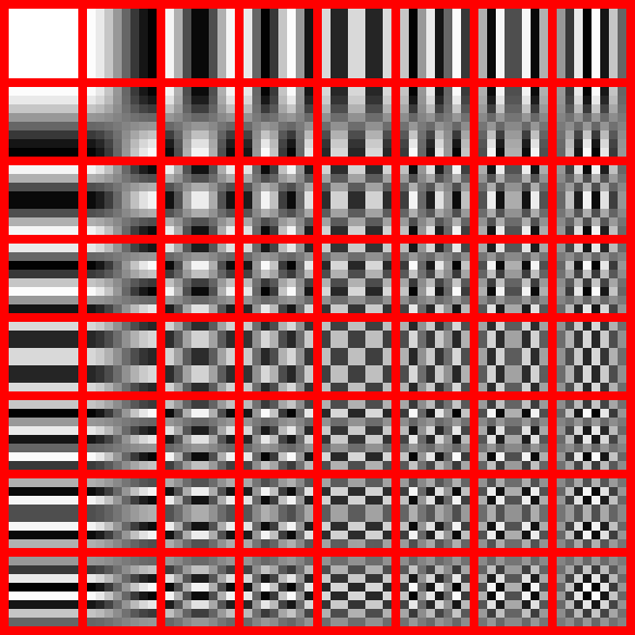
As you've mentioned, dct2 and idct2 will do most of the job for you. The question that remains is then: What is high frequency and what is low frequency content? The coefficients after the 2 dimensional transform will actually represent two frequencies each (one in x- and one in y-direction). The following figure shows the bases for each coefficient in an 8x8 discrete cosine transform:

Therefore, that question of low vs. high can be answered in different ways. A common way, which is also used in the JPEG encoding, proceeds diagonally from zero-frequency downto the max as shown above. As we can see in the following example that is mostly motivated because natural images are largely located in the "top left" corner of "low" frequencies. It is certainly worth looking at the result of dct2 and play around with the actual choice of your regions for high and low.

In the following I'm dividing the spectrum diagonally and also plotting the DCT coefficients - in logarithmic scale because otherwise we would just see one big peak around (1,1). In the example I'm cutting far above half of the coefficients (adjustible with cutoff) we can see that the high-frequency part still contains some relevant image information. If you set cutoff to 0 or below only noise of small amplitude will be left.

%// Load an image
Orig = double(imread('rice.png'));
%// Transform
Orig_T = dct2(Orig);
%// Split between high- and low-frequency in the spectrum (*)
cutoff = round(0.5 * 256);
High_T = fliplr(tril(fliplr(Orig_T), cutoff));
Low_T = Orig_T - High_T;
%// Transform back
High = idct2(High_T);
Low = idct2(Low_T);

%// Plot results
figure, colormap gray
subplot(3,2,1), imagesc(Orig), title('Original'), axis square, colorbar 
subplot(3,2,2), imagesc(log(abs(Orig_T))), title('log(DTC(Original))'),  axis square, colorbar

subplot(3,2,3), imagesc(log(abs(Low_T))), title('log(DTC(LF))'), axis square, colorbar
subplot(3,2,4), imagesc(log(abs(High_T))), title('log(DTC(HF))'), axis square, colorbar

subplot(3,2,5), imagesc(Low), title('LF'), axis square, colorbar
subplot(3,2,6), imagesc(High), title('HF'), axis square, colorbar

(*) Note on tril: The lower triangle-function operates with respect to the mathematical diagonal from top-left to bottom-right, since I want the other diagonal I'm flipping left-right before and afterwards.

Also note that this kind of operations are not usually applied to entire images, but rather to blocks of e.g. 8x8. Have a look at blockproc and this article.

这篇关于使用DCT将图像分解为两个频率分量？的文章就介绍到这了，希望我们推荐的答案对大家有所帮助，也希望大家多多支持IT屋！