如何从 ISI Web of Knowledge 中检索有关期刊的信息? [英] How to retrieve informations about journals from ISI Web of Knowledge?

问题描述

我正在研究文章的预测引用计数.我的问题是我需要来自 ISI Web of Knowledge 的期刊信息.他们年复一年地收集这些信息(期刊影响因子、特征因子……)，但无法一次下载所有一年期期刊信息.只有标记所有"选项，它总是标记列表中的前 500 个期刊(然后可以下载此列表).我正在用 R 对这个项目进行编程.所以我的问题是，如何一次或以高效整洁的方式检索这些信息?谢谢你的任何想法.

解决方案

我使用 上的一个稍大的项目):

# 设置浏览器和硒图书馆(开发工具)install_github("ropensci/rselenium")图书馆(RSelenium)检查服务器()启动服务器()remDr <- remoteDriver()remDr$open()# 去 http://apps.webofknowledge.com/# 按期刊细化搜索...也许是主题"中的 arch?eolog*# then: '研究领域' ->考古学->提炼# then: '文档类型' ->文章 ->提炼# then: '来源标题' ->选择你最喜欢的期刊 ->提炼# 必须有 <10k 结果才能启用引文数据# 点击顶部的创建引文报告"选项卡# 手动执行第一页以设置保存文件"和自动执行此操作"，# 然后让循环做之后的工作# 在运行循环之前，获取我们已经保存的第一页的 URL，# 并粘贴到下一行，每次运行的 URL 都会不同remDr$navigate("http://apps.webofknowledge.com/CitationReport.do?product=UA&search_mode=CitationReport&SID=4CvyYFKm3SC44hNsA2w&page=1&cr_pqid=7&viewType=summary")

这是从接下来的几百页 WOS 结果中自动收集数据的循环......

# 循环获取每页结果的引文数据，每次迭代都会保存一个txt文件，我使用selectorgadget来检查css id，它们可能因您而异.for(i 在 1:1000){# 点击保存到文本文件"结果 <- 尝试(webElem <- remDr$findElement(using = 'id', value = "select2-chosen-1"));if(class(result) == "try-error") next;webElem$clickElement()# 在弹出的窗口点击发送"结果 <- 尝试(webElem <- remDr$findElement(using = "css", "span.quickoutput-action"));if(class(result) == "try-error") next;webElem$clickElement()# 刷新页面以消除弹出窗口remDr$refresh()# 前进到下一页结果结果 <- 尝试(webElem <- remDr$findElement(using = 'xpath', value = "(//form[@id='summary_navigation']/table/tbody/tr/td[3]/a/i)[2]"));if(class(result) == "try-error") next;webElem$clickElement()打印(一)}# 有很多重复，但下面的代码会删除它们# 将文件夹复制到您的硬盘驱动器，并编辑下面的 setwd 行# 匹配包含数百个文本文件的文件夹的位置.

将所有文本文件读入 R...

# 手动将它们移动到自己的文件夹中setwd("/home/two/Downloads/WoS")# 获取文本文件名my_files <- list.files(pattern = ".txt")# 创建列表对象来存储 R 中的所有文本文件my_list <- vector(mode = "list", length = length(my_files))# 遍历文件名并将每个文件读入列表my_list <- lapply(seq(my_files), function(i) read.csv(my_files[i],跳过 = 4,头=真，comment.char = " "))# 检查它是否有效my_list[1:5]

将抓取的数据帧列表合并为一个大数据帧

# 使用 data.table 来提高速度install_github("rdatatable/data.table")图书馆(数据表)my_df <- rbindlist(my_list)设置键(my_df)# 只过滤几列以简化my_cols <- c('Title', 'Publication.Year', 'Total.Citations', 'Source.Title')my_df <- my_df[,my_cols, with=FALSE]# 删除重复项my_df <- 唯一(my_df)#我们有什么期刊?独特的(my_df$Source.Title)

为期刊名称制作缩写，使文章标题全部大写以备绘图...

# 获取名称long_titles <- as.character(unique(my_df$Source.Title))# 自动获取缩写，也许不是显而易见的，但它很快short_titles <- unname(sapply(long_titles, function(i){theletters = strsplit(i,'')[[1]]wh = c(1,which(theletters == ' ') + 1)字母[wh]粘贴(字母[wh]，折叠='')}))# 手动消除现在只有A"作为短名称的期刊的歧义short_titles[short_titles == "A"] <- c("AMTRY", "ANTQ", "ARCH")# 删除 'NA' 这样它就不会与实际的日志混淆short_titles[short_titles == "NA"] <- ""# 给大表添加缩写期刊 <- data.table(Source.Title = long_titles,short_title = short_titles)setkey(journals) # 需要一个键来合并my_df <-合并(my_df，期刊，by = 'Source.Title')# 文章标题全部大写，便于阅读my_df$Title <- toupper(my_df$Title)## 创建新的十年"列# 首先制作一个查找表，得到每一年的十年年 1 <- 1900:2050my_seq <- seq(year1[1], year1[length(year1)], by = 10)indx <- findInterval(year1, my_seq)ind <- seq(1, length(my_seq), by = 1)labl1 <- paste(my_seq[ind], my_seq[ind + 1], sep = "-")[-42]dat1 <- data.table(data.frame(Publication.Year = year1,十年 = labl1[indx],stringsAsFactors = FALSE))setkey(dat1, 'Publication.Year')# 将十年列合并到 my_df 上my_df <-合并(my_df，dat1，by = 'Publication.Year')

按出版年代查找被引用次数最多的论文...

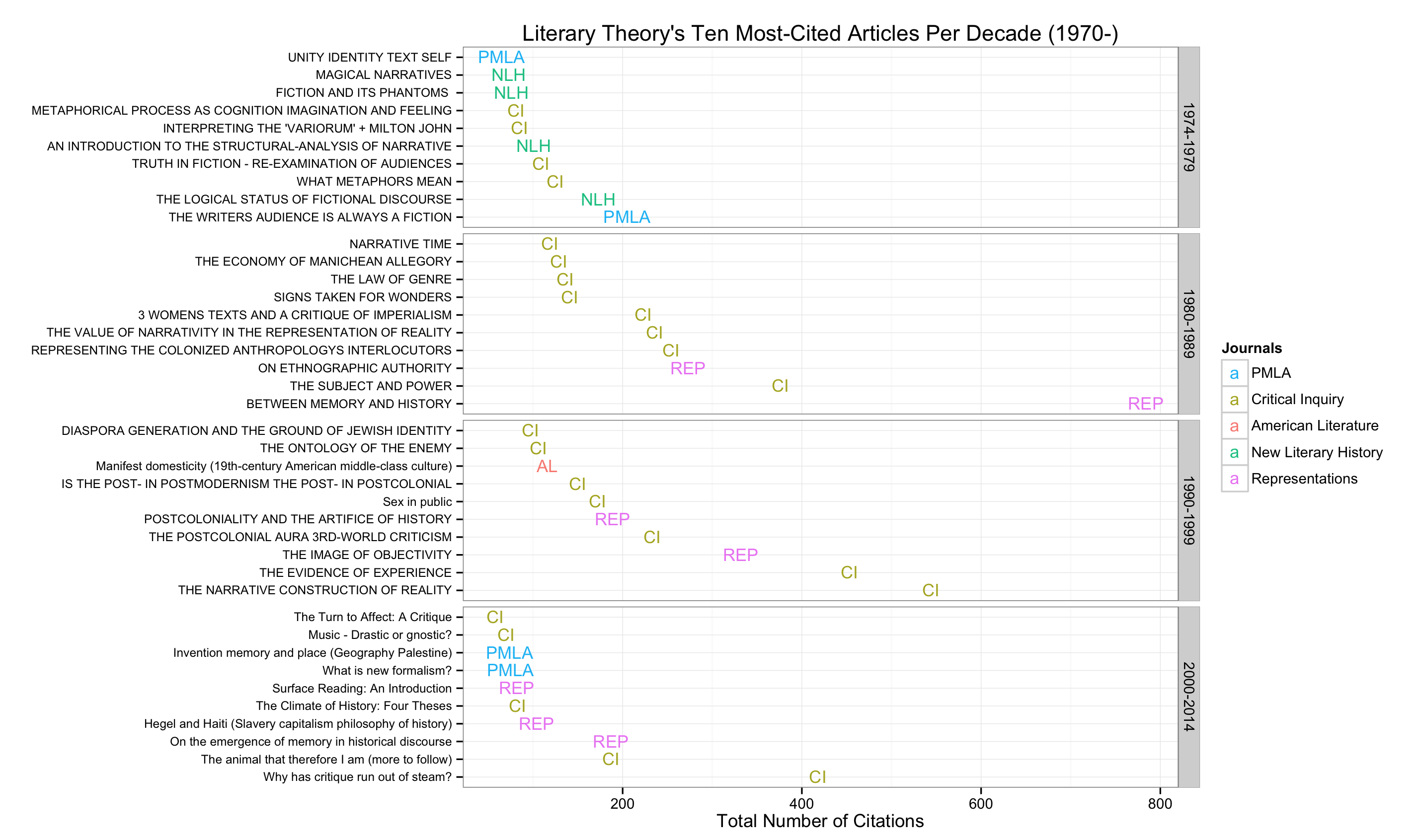
df_top <- my_df[ave(-my_df$Total.Citations, my_df$decade, FUN = rank) <= 10, ]# 检查这个 df_top 表非常有趣.

以类似于 Kieran 的风格绘制情节，此代码来自 Jonathan Goodwin，他也为他的领域复制了情节(Jonathan Goodwin="http://jgoodwin.net/lit-cites.png">1, 2)

######## 来自乔纳森古德温的绘制代码################## http://jgoodwin.net/######### 数据格式:Title、Total.Citations、decade、Source.Title# 作家观众总是虚构的，205,1974-1979,PMLA图书馆(ggplot2)ws <- df_topws <- ws[order(ws$decade,-ws$Total.Citations),]ws$Title <- factor(ws$Title, levels = unique(ws$Title)) #为了保持情节的顺序，也许还有另一种方法可以做到这一点g <- ggplot(ws, aes(x = Total.Citations,y = 标题，标签 = short_title,组 = 十年，颜色 = short_title))g <- g + geom_text(size = 4) +facet_grid (十年 ~.,下降=真，比例=free_y")+theme_bw(base_family="Helvetica") +主题(axis.text.y=element_text(size=8)) +xlab("科学引文数量") + ylab("") +labs(title="考古学每十年 (1970-) 被引用次数最多的十篇文章"，大小=7) +scale_colour_discrete(name="Journals")g #adjust 调整大小等.

情节的另一个版本，但没有代码:http://charlesbreton.ca/?page_id=179

I am working on some work of prediction citation counts for articles. The problem I have is that I need information about journals from ISI Web of Knowledge. They're gathering these information (journal impact factor, eigenfactor,...) year by year, but there is no way to download all one-year-journal-informations at once. There's just option to "mark all" which marks always first 500 journals in the list (this list then can be downloaded). I am programming this project in R. So my question is, how to retrieve this information at once or in efficient and tidy way? Thank you for any idea.

解决方案

I used RSelenium to scrape WOS to get citation data and make a plot similar to this one by Kieran Healy (but mine was for archaeology journals, so my code is tailored to that):

Here's my code (from a slightly bigger project on github):

# setup broswer and selenium
library(devtools)
install_github("ropensci/rselenium")
library(RSelenium)
checkForServer()
startServer()
remDr <- remoteDriver()
remDr$open()
# go to http://apps.webofknowledge.com/
# refine search by journal... perhaps arch?eolog* in 'topic'
# then: 'Research Areas' -> archaeology -> refine
# then: 'Document types' -> article -> refine
# then: 'Source title' -> choose your favourite journals -> refine
# must have <10k results to enable citation data
# click 'create citation report' tab at the top
# do the first page manually to set the 'save file' and 'do this automatically', 
# then let loop do the work after that

# before running the loop, get URL of first page that we already saved,
# and paste in next line, the URL will be different for each run
remDr$navigate("http://apps.webofknowledge.com/CitationReport.do?product=UA&search_mode=CitationReport&SID=4CvyYFKm3SC44hNsA2w&page=1&cr_pqid=7&viewType=summary")

Here's the loop to automate collecting data from the next several hundred pages of WOS results...

# Loop to get citation data for each page of results, each iteration will save a txt file, I used selectorgadget to check the css ids, they might be different for you.
for(i in 1:1000){
  # click on 'save to text file'
  result <- try(
    webElem <- remDr$findElement(using = 'id', value = "select2-chosen-1")
  ); if(class(result) == "try-error") next;
  webElem$clickElement()
  # click on 'send' on pop-up window
  result <- try(
    webElem <- remDr$findElement(using = "css", "span.quickoutput-action")
  ); if(class(result) == "try-error") next;
  webElem$clickElement()
  # refresh the page to get rid of the pop-up
  remDr$refresh()
  # advance to the next page of results
  result <- try(
    webElem <- remDr$findElement(using = 'xpath', value = "(//form[@id='summary_navigation']/table/tbody/tr/td[3]/a/i)[2]")
  ); if(class(result) == "try-error") next;
  webElem$clickElement()
  print(i) 
}

# there are many duplicates, but the code below will remove them
# copy the folder to your hard drive, and edit the setwd line below
# to match the location of your folder containing the hundreds of text files.

Read all text files into R...

# move them manually into a folder of their own
setwd("/home/two/Downloads/WoS")
# get text file names
my_files <- list.files(pattern = ".txt")
# make list object to store all text files in R
my_list <- vector(mode = "list", length = length(my_files))
# loop over file names and read each file into the list
my_list <- lapply(seq(my_files), function(i) read.csv(my_files[i], 
                                                      skip = 4, 
                                                      header = TRUE,                            
                                                      comment.char = " "))
# check to see it worked
my_list[1:5]

Combine list of dataframes from the scrape into one big dataframe

# use data.table for speed
install_github("rdatatable/data.table")
library(data.table)
my_df <- rbindlist(my_list)
setkey(my_df)
# filter only a few columns to simplify
my_cols <- c('Title', 'Publication.Year', 'Total.Citations', 'Source.Title')
my_df <- my_df[,my_cols, with=FALSE]
# remove duplicates
my_df <- unique(my_df)
# what journals do we have?
unique(my_df$Source.Title)

Make abbreviations for journal names, make article titles all upper case ready for plotting...

# get names
long_titles <- as.character(unique(my_df$Source.Title))
# get abbreviations automatically, perhaps not the obvious ones, but it's fast
short_titles <- unname(sapply(long_titles, function(i){
  theletters = strsplit(i,'')[[1]]
  wh = c(1,which(theletters  == ' ') + 1)
  theletters[wh]
  paste(theletters[wh],collapse='') 
}))
# manually disambiguate the journals that now only have 'A' as the short name                         
short_titles[short_titles == "A"] <- c("AMTRY", "ANTQ", "ARCH")
# remove 'NA' so it's not confused with an actual journal
short_titles[short_titles == "NA"] <- ""
# add abbreviations to big table
journals <- data.table(Source.Title = long_titles, 
                       short_title = short_titles)
setkey(journals) # need a key to merge
my_df <- merge(my_df, journals, by = 'Source.Title')
# make article titles all upper case, easier to read
my_df$Title <- toupper(my_df$Title)


## create new column that is 'decade'
# first make a lookup table to get a decade for each individual year
year1 <- 1900:2050
my_seq <- seq(year1[1], year1[length(year1)], by = 10)
indx <- findInterval(year1, my_seq)
ind <- seq(1, length(my_seq), by = 1)
labl1 <- paste(my_seq[ind], my_seq[ind + 1], sep = "-")[-42]
dat1 <- data.table(data.frame(Publication.Year = year1, 
                              decade = labl1[indx], 
                              stringsAsFactors = FALSE))
setkey(dat1, 'Publication.Year')
# merge the decade column onto my_df
my_df <- merge(my_df, dat1, by = 'Publication.Year')

Find the most cited paper by decade of publication...

df_top <- my_df[ave(-my_df$Total.Citations, my_df$decade, FUN = rank) <= 10, ] 

# inspecting this df_top table is quite interesting.

Draw the plot in a similar style to Kieran's, this code comes from Jonathan Goodwin who also reproduced the plot for his field (1, 2)

######## plotting code from from Jonathan Goodwin ##########
######## http://jgoodwin.net/ ########

# format of data: Title, Total.Citations, decade, Source.Title
# THE WRITERS AUDIENCE IS ALWAYS A FICTION,205,1974-1979,PMLA

library(ggplot2)
ws <- df_top

ws <-  ws[order(ws$decade,-ws$Total.Citations),]
ws$Title <- factor(ws$Title, levels = unique(ws$Title)) #to preserve order in plot, maybe there's another way to do this

g <- ggplot(ws, aes(x = Total.Citations, 
                    y = Title, 
                    label = short_title, 
                    group = decade, 
                    colour = short_title))

g <- g + geom_text(size = 4) + 
  facet_grid (decade ~.,
              drop=TRUE,
              scales="free_y") + 
  theme_bw(base_family="Helvetica") +
  theme(axis.text.y=element_text(size=8)) +
  xlab("Number of Web of Science Citations") + ylab("") +
  labs(title="Archaeology's Ten Most-Cited Articles Per Decade (1970-)", size=7) + 
  scale_colour_discrete(name="Journals")

g #adjust sizing, etc.

Another version of the plot, but with no code: http://charlesbreton.ca/?page_id=179

这篇关于如何从 ISI Web of Knowledge 中检索有关期刊的信息?的文章就介绍到这了，希望我们推荐的答案对大家有所帮助，也希望大家多多支持IT屋！